ARCH 655 | Project 2

An experimental study on Genetic algorithm performance  for building form optimization

1- Summary

The genetic algorithm using the Galapagos component of Grasshopper is used to find the optimized form of a building based on the total energy use. On the other hand, a large number of uniform-random cases are simulated, and among them, the best result based on the total energy use will be taken out.

Then the two solutions, GA best solution, and uniform-random best solution are compared in terms of accuracy, time and number of iterations.

2- Project Introduction

A genetic algorithm (GA) is a heuristic algorithm that is inspired by Charles Darwin's theory of natural evolution. This algorithm reflects the process of natural selection where the fittest individuals are selected for reproduction in order to produce offspring of the next generation. GA first, builds a population by random genomes. Then at the next step, it evaluates each result in the initial population and selectively breeds to form the next generation. And this will be repeated until the GA possibly reach the solution.

Galapagos in Grasshopper is developed by David Rutten with the intention of providing a generic platform for non-programmers to apply Evolutionary Algorithms on a wide variety of problems. Here, in this project, I am going to use Galapagos to find the optimized form of a building based on total energy use. 

I will be running an optimization on building the 2D shape with respect to building energy use. The building shape is the independent variable (Genomes) and total building energy use will be the dependent value (Fitness). The form of the building is changing in a determined range, in other words, a certain structure will remain consistent in all shapes and only four parameters, X1, X2, X3, X4 will be changing. The area of all forms will remain unchanged and is equal to the dotted rectangular area.

And these are merely mirrored to form the whole building perimeter.

Here are some resulted shapes that are different in 4 parameters:

The area remains equal to the dotted rectangle area which is a*b. 

For meeting constant area condition, a relation must be set between the parameters as following:

The goal is to assess the performance of evolutionary solver in comparison to uniformly random selection points to get the optimized solution.

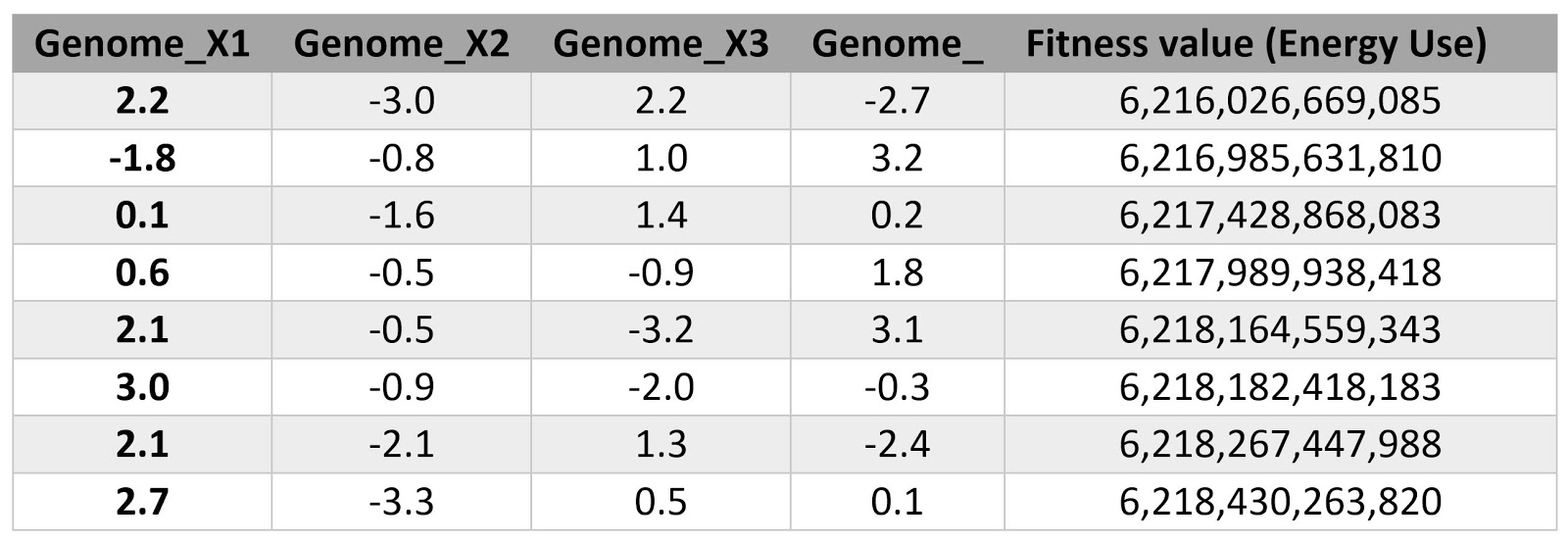
In this regard, 500 random-uniform sets of values have picked for X1, X2, X3, and X4 meeting the above-mentioned relation. Then the results are simply sorted, and the lowest energy use has selected as an optimized solution. The following table shows the top 20 results. The best result among the 500 cases is -2.2, -1,4, 2.1, 3.0 for X1, X2, X3, and X4 respectively.

On the other hand, a similar range(-3.5:3.5) is dedicated to GA as genomes.

For meeting the constant area condition, a conditional expression has inserted into the algorithm to limit the affecting genomes.

If the condition is met, then the energy simulation would run otherwise it takes a bypass and yield a very out ranged value for energy use/fitness. This way unacceptable values for X1, X2, X3, and X4 will be practically taken out from the GA results.

If we allow for 3 decimal places in the genomes it means we can generate almost 311,169,600,000,000 (or 310 trillion) unique combinations of genomes. In our case that genomes represent the length in meter, more than one decimal is enough. So, there would be 3,111,696 (or 3 million) unique combinations for X1, X2, X3, and X4.

It is worth noting that no time is spent on unnecessary simulation. And the total time of GA processing will be due to the time spent on processing of the desired genomes. The time spent by GA processing as well as the reliability of the answer and number of required iterations will be compared to the time spent on energy simulation of 500 uniform-random cases.

The GA model contains four variables, meaning that there are four values that can change. In Evolutionary Computing we refer to variables as genes. As we change Gene X1, the state of the model changes and it either becomes better or worse in terms of building energy use. So as Gene X1 changes, the fitness of the entire model goes up or down. But for every value of X1, we can also vary Gene X2, X3, and X4, resulting in better or worse combinations of X1, X2, X3, and X4. Every combination of X1, X2, X3, and X4 results in particular fitness, and this fitness is expressed as the total building energy use. For energy use simulation Honeybee plug-in has been used in Grasshopper, which uses the Energy Plus motor engine for energy analysis. It is the job of the solver to find the lowest energy use in this problem and then yield the resulting genes.

As the solver starts it has no idea about the actual value of the fitness of the energy use. So, the initial step of the solver is to generate an initial pool of solutions or in other words, to populate the fitness values with a random collection of genomes.

In our case, a genome could for example be {X1=2.3, X2=-3.5, X3=1.5, X4=-0.6}. The solver will then evaluate the fitness for these random genomes, giving us the energy use value of 1,762,816 (J). it is important the initial value.

Once the model figured out how to fit the picked random genomes are, in other words how the energy use of the red dots is like, it will make a hierarchy from lowest to highest energy use. The genomes resulted in lower energy use are closer to potential best genes. Therefore, we can kill off the worst-performing ones and focus on the remainder.

It is not good enough to simply pick the best performing genome from the initial population. Since all the genomes in Generation 0 were picked at random, it is quite unlikely that any of them be the optimized answer. What GA will do is breed the best performing genomes in Generation 0 to create Generation 1 and so on.

We now have a new population, which is no longer completely random, and which is already starting to cluster around the relatively lowest energy use-values. All GA has to do is to repeat the above steps, kill off the worst-performing genomes, and breed the best-performing genomes, until we have reached the lowest energy use.

GA solution is a result of random-based iterations, following evolutionary improvement. So, since both methods, GA and uniform-random are random, the procedure should be repeated multiple times to have a better estimate of their performance. Here for this project due to the time limit, the comparison is done based on a one-time iteration.

3-Discussion

It should be noted that the Evolutionary Algorithm does not guarantee a solution. Unless a predefined 'good-enough' value is specified, the process will tend to run on indefinitely, never reaching the answer, or, having reached it, not recognizing it for what it is.

Genetic algorithms cannot solve any problems. Fitness function not increasing is common and it is referred to as the stalling effect. Problems like this are typically very difficult to solve by evolutionary solving, as the solution tends to get stuck in local optima.

In this problem, we are facing a landscape that has a high degree of noise or chaos. A landscape may be continuous and yet feature so much detail that it becomes impossible to make any intelligible pronunciations regarding the fitness of a local patch:

In a landscape like this, parents may both be very similar, and both be very fit, but when they mate the offspring might end up in one of the fissures. A landscape like this defies navigation.